Data Server's SQL dialect

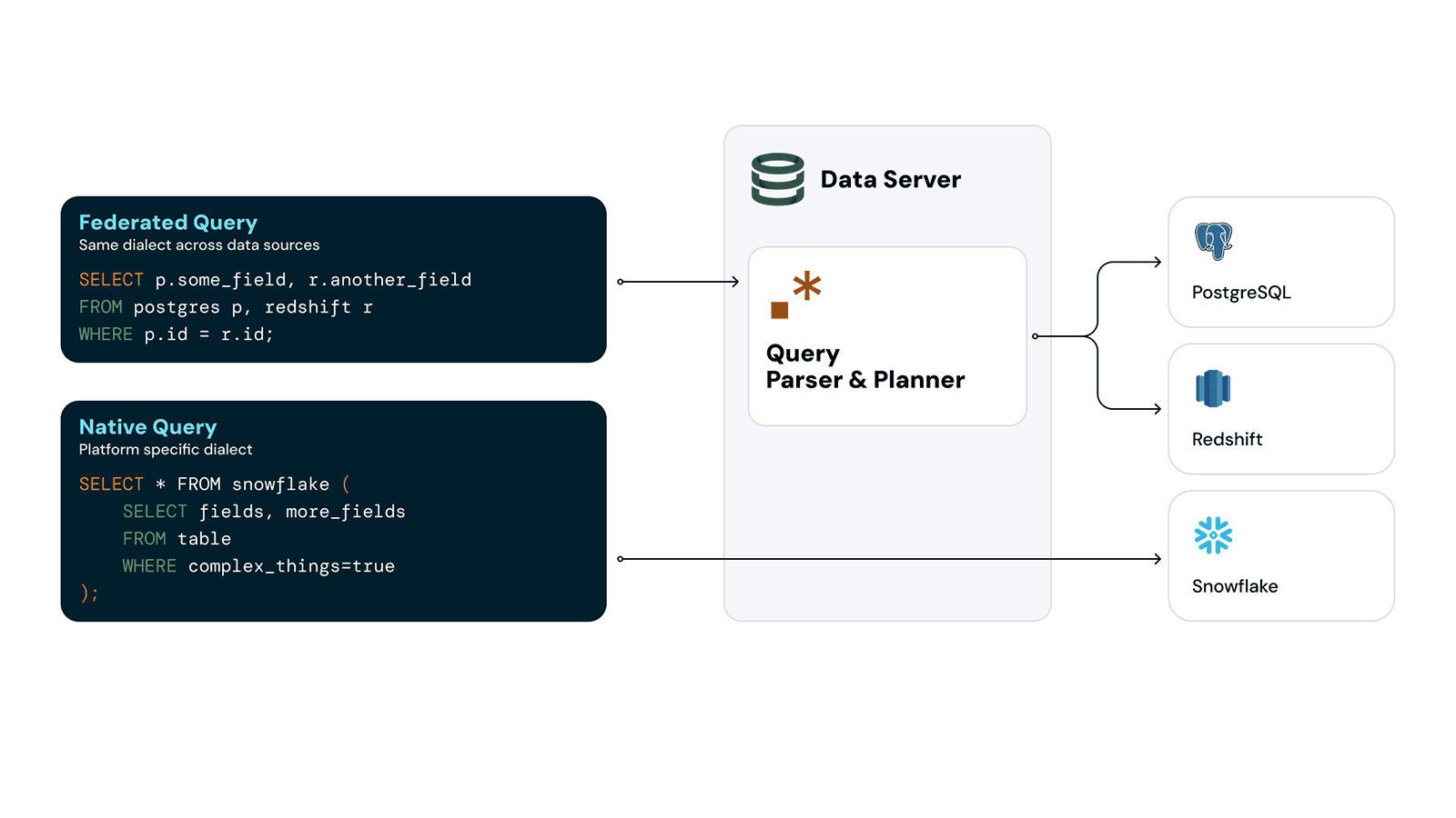
Data Server implements a federated query engine that allows you to query all supported databases and file-based storage with single SQL dialect. The syntax follows conventions of PostgreSQL and MysQL. This section describes the syntax, conventions and gives tips for effective queries.

Common conventions

Data Server and the documentation follows these conventions:

• Reserved words are capitalized. For example: SELECT.
• Square brackets [] indicate optional clauses.
• Curly brackets {} indicate logical or choices with the options separated by |. For example {x | y | z}.
• Identifiers (databases, tables, and column names) with special characters or reserved words must be enclosed with backticks `, for example SELECT * FROM `select` WHERE `select`.id > 100;
• String values are represented by single and double quotes, for example SELECT * FROM table_name WHERE table_name.column_name = 'string'; or ... table_name.column_name = "string";
• SQL statements can be nested with parentheses, like this SELECT * FROM (SELECT * FROM table_name WHERE table_name.column_name = 'string');

Data sources

To manage data sources within the Sema4.ai Data Server, you can perform the following operations:

Connecting to a Data Source

To establish a connection to an external data source, use the CREATE DATABASE statement. This command links the Data Server to your specified data source, enabling seamless data access without copying the data over.

CREATE DATABASE database_name
WITH ENGINE = 'engine_name',
PARAMETERS = {
    "host": "host_address",
    "port": port_number,
    "user": "username",
    "password": "password",
    "database": "database_name"
};

Data Server currently supports PostgreSQL, Redsihft and Snowflake with more supported sources coming soon. Replace the placeholders with your data source's specific details (which may differ per data source type). For example, to connect to a PostgreSQL database:

CREATE DATABASE public_demo
WITH ENGINE = 'postgres',
PARAMETERS = {
    "host": "data-access-public-demo-instance-1.chai8y6e2qqq.us-east-2.rds.amazonaws.com",
    "port": 5432,
    "user": "demo_user",
    "password": "password",
    "database": "xyzxyzxyz"
};

Listing available data sources

To view all data sources currently connected to the Sema4.ai Data Server, execute the SHOW DATABASES command. This will display a list of all available databases.

SHOW DATABASES;

Selecting data source

To specify a particular data source for your queries, use the USE statement followed by the integration name. This sets the context for subsequent operations to the chosen data source.

USE integration_name;

After setting the context, you can perform queries on the tables within that data source.

For example:

USE public_demo;
SELECT * FROM demo_customers LIMIT 10;

Disconnect data source

Disconnecting a data source can be done with DROP statement. Note that this is NOT removing the data from your database, but removing the link in the Data Server.

DROP DATABASE IF EXISTS public_demo;

Tables, Views, Files

To manage tables, views, and files within the Sema4.ai Data Server, you can perform the following operations:

Creating Tables, Views, and Files

To create a table, use the CREATE TABLE statement. This command allows you to define a new table structure and optionally populate it with data from a query. You can also create views and files using similar commands tailored to each type.

CREATE TABLE integration_name.table_name (
  column_name data_type,
  ...
);

For views, use the CREATE VIEW statement to define a virtual table based on a query.

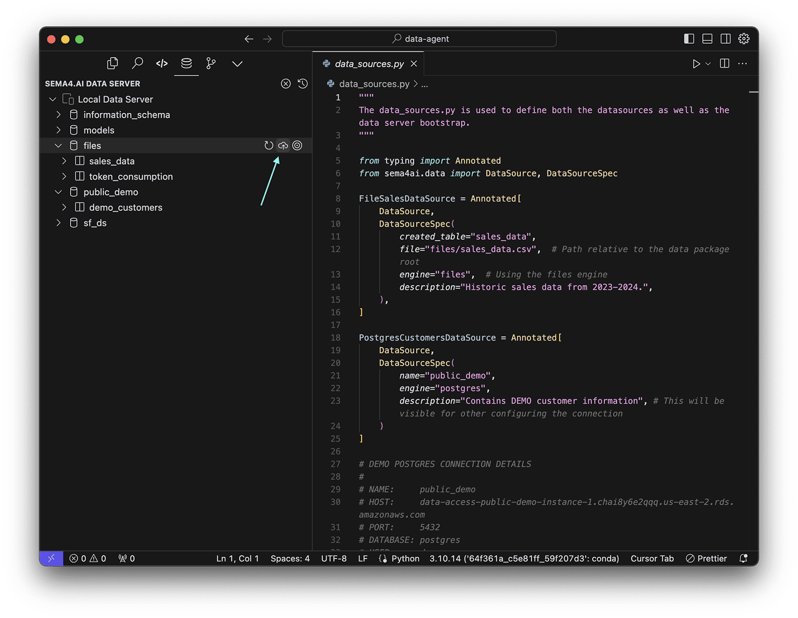
Files can be uploaded and managed easiest with the VS Code extension features, like this:

Removing Tables, Views, and Files

To remove a view, or file, use the DROP statement. This command deletes the specified data structure from the Data Server, freeing up resources and maintaining data organization.

DROP VIEW IF EXISTS integration_name.view_name;
DROP FILE IF EXISTS integration_name.file_name;

Querying Tables, Views, and Files

To retrieve data from tables, views, and files within the Sema4.ai Data Server, use the SELECT statement. This command allows you to specify the data you wish to get, applying filters and conditions as needed to refine your results.

SELECT column_name1, column_name2
FROM integration_name.table_name
WHERE condition;

For views, the process is similar, as they act like virtual tables. You can query them using the same SELECT syntax, leveraging the predefined logic of the view to simplify complex queries.

SELECT *
FROM integration_name.view_name
WHERE condition;

When querying files, ensure that the file format and structure are compatible with your query requirements. The Data Server supports various file types, allowing you to perform ad-hoc queries directly on the data.

SELECT *
FROM files.file_name
WHERE condition;

or when it comes to Excel files, also refer to the sheet:

SELECT *
FROM files.file_name.sheet_name
WHERE condition;

These querying capabilities enable you to access and analyze your data efficiently, providing the insights needed to drive informed business decisions.

Joining Tables Across Data Sources

The Data Server allows you to join tables from different data sources, enabling complex queries and data integration. Use the JOIN clause in your SQL statements to combine data from multiple tables, even if they reside in separate integrations.

SELECT *
FROM integration1.table1 AS t1
JOIN integration2.table2 AS t2
ON t1.common_field = t2.common_field;

This capability enhances data analysis by providing a unified view of disparate data sets, facilitating comprehensive insights and decision-making.

Native queries

In the Sema4.ai Data Server, you can execute native SQL queries specific to your database engine, providing flexibility and control over your data operations and bypassing the federeted query engine. This allows you to run more complex queries using platform specific features.

Here's how you can work with native queries:

Once your data source is connected, you can execute native SQL queries by nesting them within a SELECT statement. This allows you to leverage the full capabilities of your database engine directly from the Data Server.

SELECT * FROM example_db (
    SELECT 
        model, 
        year, 
        price, 
        transmission, 
        mileage, 
        fueltype, 
        mpg, -- miles per gallon
        ROUND(CAST((mpg / 2.3521458) AS numeric), 1) AS kml, -- kilometers per liter
        (date_part('year', CURRENT_DATE)-year) AS years_old, -- age of a car
        COUNT(*) OVER (PARTITION BY model, year) AS units_to_sell, -- units sold per model per year
        ROUND((CAST(tax AS decimal) / price), 3) AS tax_div_price -- tax to price ratio
    FROM demo_data.used_car_price
);

Easiest way to start using native queries is from the action template we provide with our extension. When bootstrapping a new action project, choose Data Access/Native Query template, and follow the readme for more details.

You can also create views based on native queries, which allows you to save complex query logic as a virtual table for easy reuse.

CREATE VIEW cars FROM example_db (
    SELECT 
        model, 
        year, 
        price, 
        transmission, 
        mileage, 
        fueltype, 
        mpg, -- miles per gallon
        ROUND(CAST((mpg / 2.3521458) AS numeric), 1) AS kml, -- kilometers per liter
        (date_part('year', CURRENT_DATE)-year) AS years_old, -- age of a car
        COUNT(*) OVER (PARTITION BY model, year) AS units_to_sell, -- units sold per model per year
        ROUND((CAST(tax AS decimal) / price), 3) AS tax_div_price -- tax to price ratio
    FROM demo_data.used_car_price
);

These capabilities enable you to perform complex data manipulations and analyses directly within the Data Server, leveraging the strengths of your existing database systems.

Standard SQL structures

Common Table Expressions

Data Server supports standard SQL syntax, including Common Table Expressions (CTEs).

CTEs are used to create temporary, named result sets that simplify complex queries, improve readability, and enable modular query design by breaking down large queries into smaller, more manageable parts.

WITH table_name1 AS (
    SELECT columns
    FROM table1 t1
    JOIN table2 t2
    ON t1.col = t2.col
),
table_name2 AS (
    SELECT columns
    FROM table1 t1
    JOIN table2 t2
    ON t1.col = t2.col
)
SELECT columns
FROM table_name1 t1
JOIN table_name2 t2
ON t1.col = t2.col;

This structure allows for clearer and more organized SQL queries by defining intermediate result sets that can be referenced in subsequent parts of the query.

CASE WHEN statement

Data Server supports standard SQL syntax, including the CASE WHEN statement.

The CASE WHEN statement is used to implement conditional logic within queries. It evaluates conditions and returns specific values based on whether each condition is true or false, enabling conditional output within SELECT, WHERE, and other clauses.

SELECT
    CASE
        WHEN a = 1 THEN a + b
        WHEN 1 + 2 = b * 2 THEN 0
        WHEN (a + b > 2 OR b < c + 3) AND a > b THEN b
        ELSE c
    END
FROM table_name;

This statement allows for dynamic decision-making within SQL queries, providing flexibility to return different results based on specified conditions.

Aggregate functions

Data Server supports standard SQL syntax, including SQL aggregate functions.

SQL aggregate functions perform calculations on a set of values and return a single result, making them ideal for summarizing or analyzing data across multiple rows. Common aggregate functions include COUNT(), SUM(), AVG(), MIN(), and MAX(). These functions are often used with GROUP BY to organize results by specific categories.

SELECT
    year,
    SUM(salary) AS annual_salary
FROM salaries
GROUP BY year;

This example demonstrates how aggregate functions can be used to calculate total salaries for each year, providing a concise summary of data grouped by the year.

Window function

Data Server supports standard SQL syntax, including SQL window functions.

Window functions in SQL perform calculations across a set of table rows related to the current row, without collapsing rows into a single result like aggregate functions do. These functions are useful for tasks such as ranking, calculating running totals, and working with moving averages. Common window functions include ROW_NUMBER(), RANK(), DENSE_RANK(), NTILE(n), LAG(), LEAD(), SUM(), and AVG().

SELECT
    a + b * (c - d) AS a,
    AVG(a) OVER (PARTITION BY b)
FROM table_name;

This example illustrates how window functions can be used to calculate averages within partitions of data, allowing for detailed analysis while maintaining the original row structure.